Running the scoreboard model

This example shows how to apply the ScoreboardModel to an ArgusII implant.

The scoreboard model is a standard baseline model of retinal prosthesis stimulation, which assumes that electrical stimulation leads to the percept of focal dots of light, centered over the visual field location associated with the stimulated retinal field location \((x_{stim}, y_{stim})\), whose spatial intensity decays with a Gaussian profile [Hayes2003], [Thompson2003]:

\[I_{score}(x,y; \rho) = \exp \Big( -\frac{(x-x_{stim})^2 + (y-y_{stim})^2}{2 \rho^2} \Big)\]

where \(\rho\) is the spatial decay constant.

Important

As pointed out by [Beyeler2019], the scoreboard model does not well account for percepts generated by epiretinal implants, where incidental stimulation of retinal nerve fiber bundles leads to elongated, ‘streaky’ percepts.

In that case, use AxonMapModel instead.

The scoreboard model can be instantiated and run in three simple steps.

1. Creating the model

The first step is to instantiate the ScoreboardModel class by calling its constructor method. The most important parameter to set is rho from the above equation (here set to 100 micrometers):

from pulse2percept.models import ScoreboardModel
model = ScoreboardModel(rho=100)

Parameters you don’t specify will take on default values. You can inspect all current model parameters as follows:

print(model)

Out:

ScoreboardModel(engine='joblib', grid_type='rectangular',
                n_jobs=-1, rho=100, scheduler='threading',
                thresh_percept=0.6065306597126334,
                verbose=True, xrange=(-20, 20),
                xystep=0.25, yrange=(-15, 15))

This reveals a number of other parameters to set, such as:

• xrange, yrange: the extent of the visual field to be simulated, specified as a range of x and y coordinates (in degrees of visual angle, or dva). For example, we are currently sampling x values between -20 dva and +20dva, and y values between -15 dva and +15 dva.
• xystep: The resolution (in dva) at which to sample the visual field. For example, we are currently sampling at 0.25 dva in both x and y direction.
• thresh_percept: You can also define a brightness threshold, below which the predicted output brightness will be zero. It is currently set to 1/sqrt(e), because that will make the radius of the predicted percept equal to rho.

In addition, you can choose the parallelization back end used to speed up simulations:

• engine:

  • ‘serial’: single-core processing (no parallelization)
  • ‘joblib’: parallelization using the JobLib library
  • ‘dask’: parallelization using the Dask library

• scheduler:

  • ‘threading’: a scheduler backed by a thread pool
  • ‘multiprocessing’: a scheduler backed by a process pool

To change parameter values, either pass them directly to the constructor above or set them by hand, like this:

model.engine = 'serial'

Then build the model. This is a necessary step before you can actually use the model to predict a percept, as it performs a number of expensive setup computations (e.g., building the spatial reference frame, calculating electric potentials):

model.build()

Out:

ScoreboardModel(engine='serial', grid_type='rectangular',
                n_jobs=-1, rho=100, scheduler='threading',
                thresh_percept=0.6065306597126334,
                verbose=True, xrange=(-20, 20),
                xystep=0.25, yrange=(-15, 15))

Note

You need to build a model only once. After that, you can apply any number of stimuli – or even apply the model to different implants – without having to rebuild (which takes time).

2. Assigning a stimulus

The second step is to specify a visual prosthesis from the implants module.

In the following, we will create an ArgusII implant. By default, the implant will be centered over the fovea (at x=0, y=0) and aligned with the horizontal meridian (rot=0):

from pulse2percept.implants import ArgusII
implant = ArgusII()

The easiest way to assign a stimulus to the implant is to pass a NumPy array that specifies the current amplitude to be applied to every electrode in the implant.

For example, the following sends 10 microamps to all 60 electrodes of the implant:

import numpy as np
implant.stim = 10 * np.ones(60)

Note

Some models can handle stimuli that have both a spatial and a temporal component. the scoreboard model cannot.

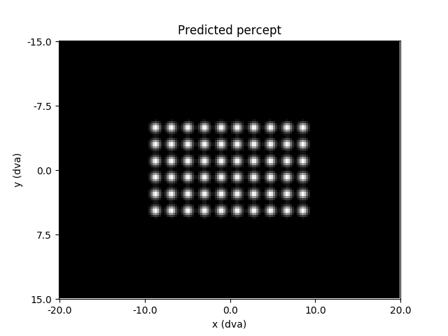
3. Predicting the percept

The third step is to apply the model to predict the percept resulting from the specified stimulus. Note that this may take some time on your machine:

percept = model.predict_percept(implant)

The resulting percept is stored in a NumPy array whose dimensions correspond to the values specified by xrange, yrange, and xystep.

The percept can be plotted using Matplotlib:

import matplotlib.pyplot as plt
plt.imshow(percept, cmap='gray')
plt.xticks(np.linspace(0, percept.shape[1], num=5),
           np.linspace(*model.xrange, num=5))
plt.xlabel('x (dva)')
plt.yticks(np.linspace(0, percept.shape[0], num=5),
           np.linspace(*model.yrange, num=5))
plt.ylabel('y (dva)')
plt.title('Predicted percept')

Out:

Text(0.5, 1.0, 'Predicted percept')