Generating simple pulses and pulse trains

This example shows how to build and visualize basic types of stimuli such as MonophasicPulse, BiphasicPulse or a PulseTrain for a given implant.

A monophasic pulse has a single phase and can be either anodic (by definition: has a positive current amplitude) or cathodic (negative current amplitude).

A biphasic pulse is generally charge-balanced for safety reasons (i.e., the net current must sum to zero over time) and defined as either anodic-first or cathodic-first.

Multiple pulses can form a pulse train.

Simplest stimulus

Stimulus is the base class to generate different types of stimuli. The simplest way to instantiate a Stimulus is to pass a scalar value which is interpreted as the current amplitude for a single electrode.

# Let's start by importing necessary modules
from pulse2percept.stimuli import (MonophasicPulse, BiphasicPulse,
                                   Stimulus, PulseTrain)

import numpy as np

stim = Stimulus(10)

Parameters we don’t specify will take on default values. We can inspect all current model parameters as follows:

print(stim)

Out:

Stimulus(data=[[10.]], electrodes=[0], metadata=None,
         shape=(1, 1), time=None)

This command also reveals a number of other parameters to set, such as:

• electrodes: We can either specify the electrodes in the source or within the stimulus. If none are specified it looks up the source electrode.
• metadata: Optionally we can include metadata to the stimulus we generate as a dictionary.

To change parameter values, either pass them directly to the constructor above or set them by hand, like this:

stim.metadata = {'name': 'A simple stimulus', 'date': '2020-01-01'}
stim

Out:

Stimulus(data=[[10.]], electrodes=[0],
         metadata={'name': 'A simple stimulus', 'date': '2020-01-01'},
         shape=(1, 1), time=None)

A monophasic pulse

We can specify the arguments of the monophasic pulse as follows:

pulse_type = 'anodic'  # anodic: positive amplitude, cathodic: negative
pulse_dur = 4.6 / 1000  # pulse duration in seconds
delay_dur = 10.0 / 1000  # pulse delivered after delay in seconds
stim_dur = 0.5  # stimulus duration in seconds (pulse padded with zeros)
time_step = 0.1 / 1000  # temporal sampling step in seconds

The sampling step time_step defines at which temporal resolution the stimulus is resolved. In the above example, the time step is 0.1 ms.

By calling Stimulus with a MonophasicPulse source, we can generate a single pulse:

monophasic_stim = Stimulus(MonophasicPulse(ptype=pulse_type, pdur=pulse_dur,
                                           delay_dur=delay_dur,
                                           stim_dur=stim_dur,
                                           tsample=time_step))
print(monophasic_stim)

Out:

Stimulus(data=[[0. 0. ... 0. 0.]], electrodes=[0],
         metadata=None, shape=(1, 5000),
         time=[0.e+00 1.e-04 ... 5.e-01 5.e-01])

Here, data is a 2D NumPy array where rows are electrodes and columns are the points in time. Since we did not specify any electrode names in MonophasicPulse, the number of electrodes is inferred from the input source type. There is only one row in the above example, denoting a single electrode.

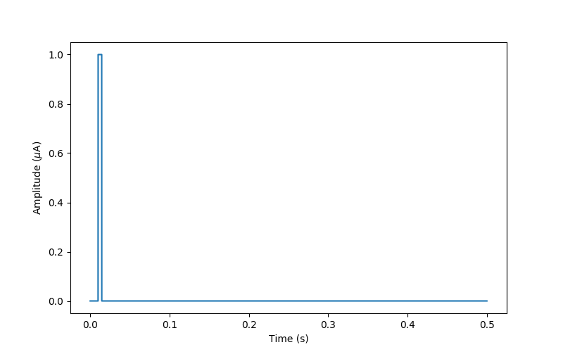
By default, the MonophasicPulse object automatically assumes a current amplitude of 1 uA.

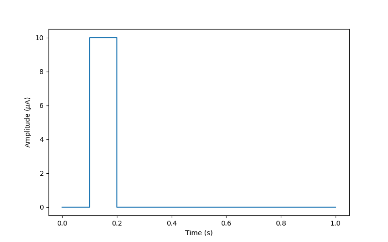
We can visualize the generated pulse using Matplotlib:

import matplotlib.pyplot as plt
fig, ax = plt.subplots(figsize=(8, 5))
ax.plot(monophasic_stim.time, monophasic_stim.data[0, :])
ax.set_xlabel('Time (s)')
ax.set_ylabel('Amplitude ($\mu$A)')

Out:

Text(0, 0.5, 'Amplitude ($\\mu$A)')

A biphasic pulse

Similarly, we can generate a biphasic pulse by changing the source of the stimulus to BiphasicPulse. This time parameter ptype can either be ‘anodicfirst’ or ‘cathodicfirst’.

# set relevant parameters
pulse_type = 'cathodicfirst'
biphasic_stim = Stimulus(BiphasicPulse(ptype=pulse_type, pdur=pulse_dur,
                                       tsample=time_step))

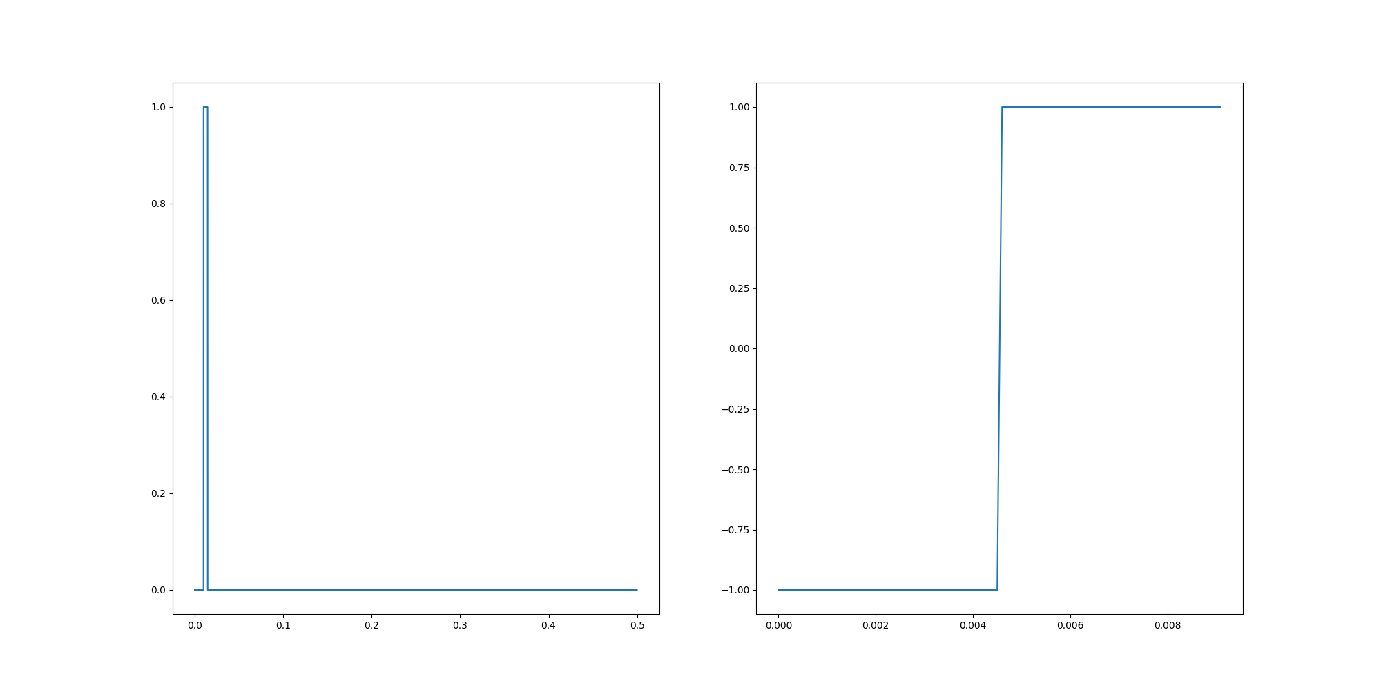
If we visualize this stimulus, we can see the difference between a monophasic and biphasic pulse:

# Create a figure with two subplots
fig, axes = plt.subplots(1, 2, figsize=(20, 10))

# First, plot monophasic pulse
axes[0].plot(monophasic_stim.time, monophasic_stim.data[0])
ax.set_xlabel('Time (s)')
ax.set_ylabel('Amplitude ($\mu$A)')

# Second, plot biphasic pulse
axes[1].plot(biphasic_stim.time, biphasic_stim.data[0])
ax.set_xlabel('Time (s)')
ax.set_ylabel('Amplitude ($\mu$A)')

Out:

Text(62.722222222222214, 0.5, 'Amplitude ($\\mu$A)')

Changing pulse amplitude

For any given pulse, we can modify the amplitude by indexing into the data row that corresponds to the desired electrode. In the above example, we only have one electrode (index 0). Let’s say we want the amplitude of the monophasic pulse to be 10 micro amps. We have two options: either change the values of the data array directly:

# get the data structure by indexing the electrode at 0
monophasic_stim.data[0] = 10*monophasic_stim.data[0]
print(monophasic_stim)

Out:

Stimulus(data=[[0. 0. ... 0. 0.]], electrodes=[0],
         metadata=None, shape=(1, 5000),
         time=[0.e+00 1.e-04 ... 5.e-01 5.e-01])

Or we can create a NumPy array and assign that to the data structure of the stimulus:

# recreate the same stimulus with an amplitude 1 microAmps.
monophasic_stim = Stimulus(MonophasicPulse(ptype='anodic', pdur=pulse_dur,
                                           delay_dur=delay_dur,
                                           stim_dur=stim_dur,
                                           tsample=time_step))
monophasic_stim.data[0] = 10*np.ones_like(monophasic_stim.data[0])
print(monophasic_stim)

Out:

Stimulus(data=[[10. 10. ... 10. 10.]], electrodes=[0],
         metadata=None, shape=(1, 5000),
         time=[0.e+00 1.e-04 ... 5.e-01 5.e-01])

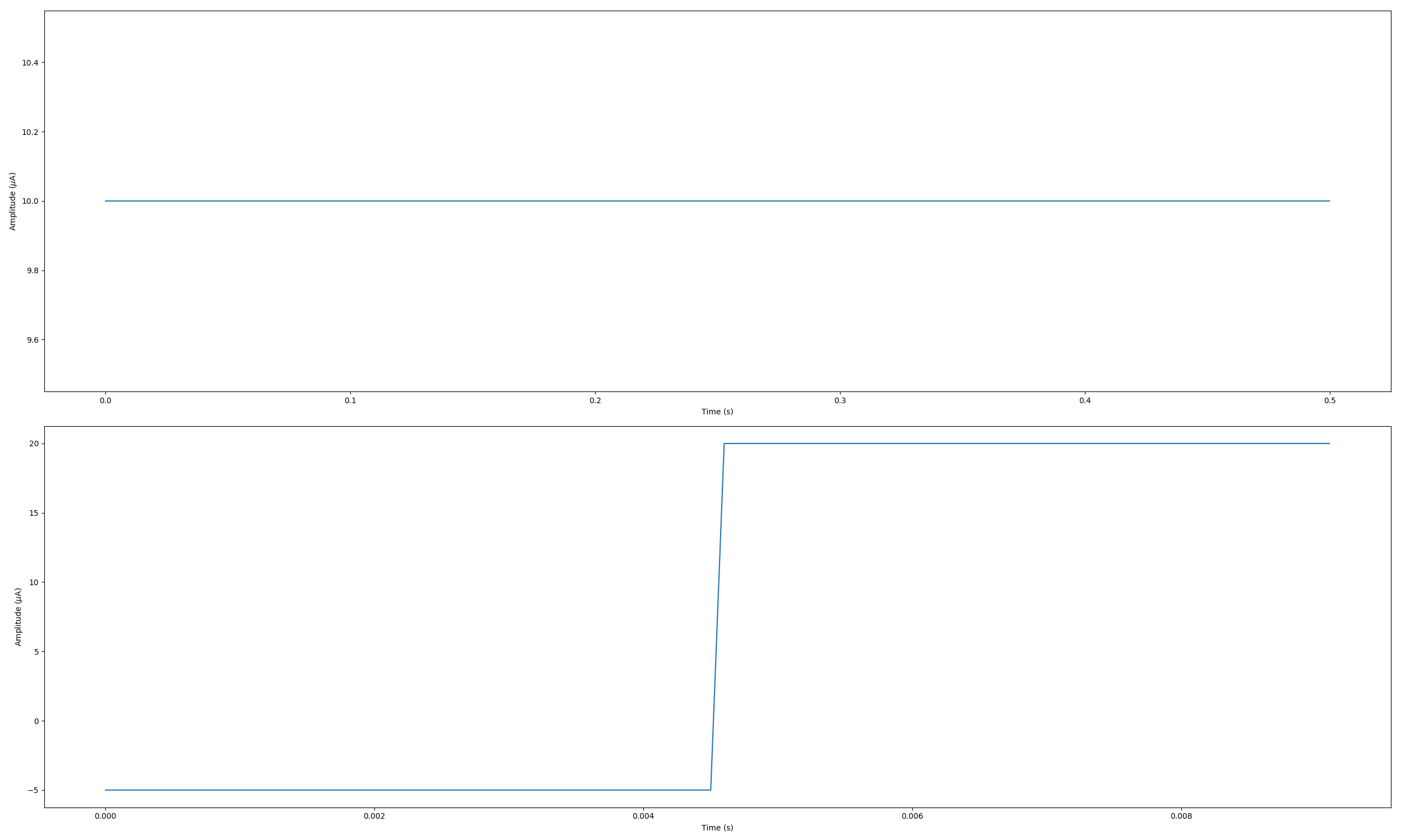
Similarly, let’s say we want the cathodic part of the biphasic pulse to be -5 micro amps, and the anodic part to be +20 micro amps (note that this stimulus wouldn’t be charge-balanced).

We first need to find the halfway point where the current switches from cathodic to anodic. To do that we first get the length of the pulse by indexing the single electrode at 0

length = len(biphasic_stim.data[0])
print(length)

# Find the halfway where cathodic turns into anodic pulse
half = int(len(biphasic_stim.data[0])/2)
print("Halfway index is", half)

# change the first half of the pulse to be 5 times larger
biphasic_stim.data[0][0:half] = 5*biphasic_stim.data[0][0:half]

# change the second half to be 20 times larger
biphasic_stim.data[0][half:length] = 20*biphasic_stim.data[0][half:length]

Out:

92
Halfway index is 46

Let’s plot the monophasic and biphasic pulses again:

# Create a figure with two subplots
fig, axes = plt.subplots(nrows=2, figsize=(25, 15))

# First, plot monophasic pulse
axes[0].plot(monophasic_stim.time, monophasic_stim.data[0])
axes[0].set_xlabel('Time (s)')
axes[0].set_ylabel('Amplitude ($\mu$A)')
# Second, plot biphasic pulse
axes[1].plot(biphasic_stim.time, biphasic_stim.data[0])
axes[1].set_xlabel('Time (s)')
axes[1].set_ylabel('Amplitude ($\mu$A)')
fig.tight_layout()

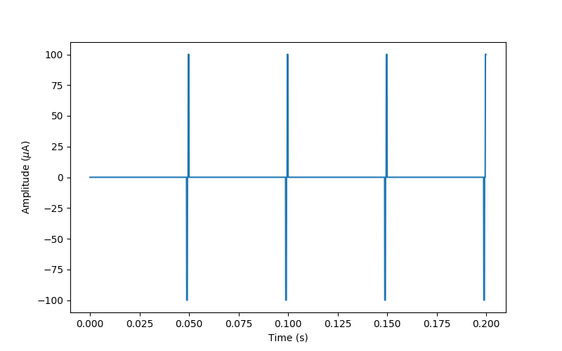
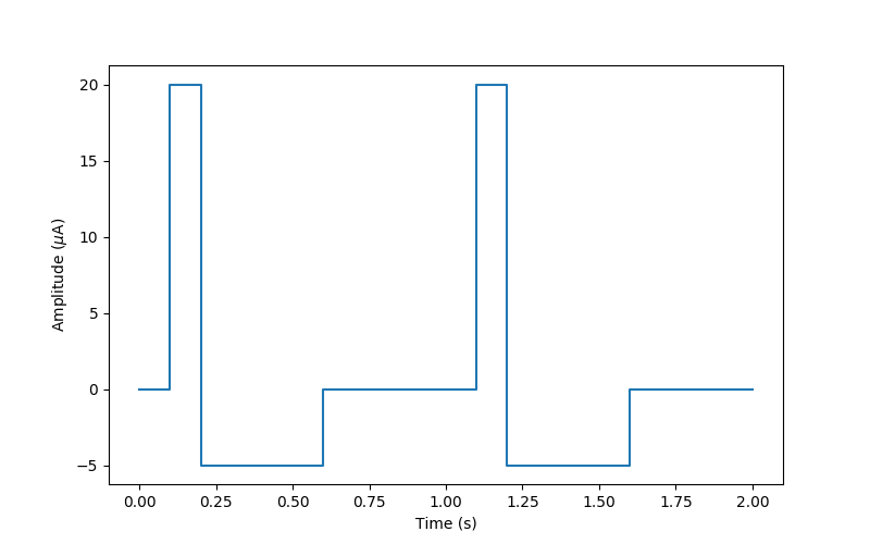
Generating standard pulse trains

The easiest way to generate a pulse train is to use the PulseTrain object, which allows for various stimulus attributes to be specified:

time_step = 0.1 / 1000  # temporal sampling in seconds
freq = 20  # frequency in Hz
amp = 100  # maximum amplitude of the pulse train in microAmps
dur = 0.2  # total duration of the pulse train in seconds
pulse_type = 'cathodicfirst'  # whether the first phase is positive or negative
pulse_order = 'gapfirst'  # whether the train starts with gap or a pulse.

# Define the pulse train with given parameters
ptrain = PulseTrain(tsample=time_step,
                    freq=freq,
                    dur=dur,
                    amp=amp,
                    pulsetype=pulse_type,
                    pulseorder=pulse_order)

# Create a new stimulus where the pulse train is the source
ptrain_stim = Stimulus(ptrain)

# Visualize:
fig, ax = plt.subplots(figsize=(8, 5))
ax.plot(ptrain_stim.time, ptrain_stim.data[0, :])
ax.set_xlabel('Time (s)')
ax.set_ylabel('Amplitude ($\mu$A)')

Out:

Text(0, 0.5, 'Amplitude ($\\mu$A)')

Alternatively, we are free to specify a discrete set of points in time and the current amplitude we would like to apply at those times.

It is important to note that the Stimulus object will linearly interpolate between specified time points. For example, the following generates a simple sawtooth stimulus:

stim = Stimulus([[0, -10, 10, -10, 10, -10, 0]],
                time=[0, 0.1, 0.3, 0.5, 0.7, 0.9, 1.0])
fig, ax = plt.subplots(figsize=(8, 5))
ax.plot(stim.time, stim.data[0, :])
ax.set_xlabel('Time (s)')
ax.set_ylabel('Amplitude ($\mu$A)')

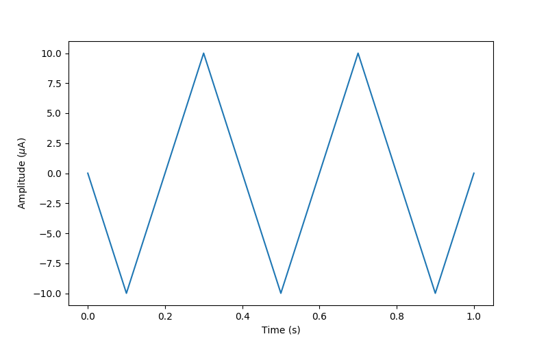
Out:

Text(0, 0.5, 'Amplitude ($\\mu$A)')

For a biphasic pulse, we need to specify both the rising edge (low-to-high transition) and falling edge (high-to-low transition) of the signal:

stim = Stimulus([[0, 0, 10, 10,  0, 0]],
                time=[0, 0.1, 0.1, 0.2, 0.2, 1.0])
fig, ax = plt.subplots(figsize=(8, 5))
ax.plot(stim.time, stim.data[0, :])
ax.set_xlabel('Time (s)')
ax.set_ylabel('Amplitude ($\mu$A)')

Out:

Text(0, 0.5, 'Amplitude ($\\mu$A)')

We can thus generate arbitrarily complex stimuli:

stim = Stimulus([[0, 0, 20, 20, -5, -5, 0, 0, 0, 20, 20, -5, -5, 0, 0]],
                time=[0, 0.1, 0.1, 0.2, 0.2, 0.6, 0.6, 1.0, 1.1, 1.1, 1.2, 1.2, 1.6, 1.6, 2.0])
fig, ax = plt.subplots(figsize=(8, 5))
ax.plot(stim.time, stim.data[0, :])
ax.set_xlabel('Time (s)')
ax.set_ylabel('Amplitude ($\mu$A)')

Out:

Text(0, 0.5, 'Amplitude ($\\mu$A)')